Navigating The Landscape Of Dimensionality Reduction: A Comprehensive Guide To UMAP Settings

Navigating the Landscape of Dimensionality Reduction: A Comprehensive Guide to UMAP Settings

Related Articles: Navigating the Landscape of Dimensionality Reduction: A Comprehensive Guide to UMAP Settings

Introduction

In this auspicious occasion, we are delighted to delve into the intriguing topic related to Navigating the Landscape of Dimensionality Reduction: A Comprehensive Guide to UMAP Settings. Let’s weave interesting information and offer fresh perspectives to the readers.

Navigating the Landscape of Dimensionality Reduction: A Comprehensive Guide to UMAP Settings

In the realm of data analysis, dimensionality reduction techniques play a pivotal role in simplifying complex datasets and extracting meaningful insights. Among these techniques, Uniform Manifold Approximation and Projection (UMAP) has emerged as a powerful and versatile tool, offering a balance between preserving global structure and revealing local details. Understanding the intricacies of UMAP settings is crucial for effectively harnessing its capabilities and achieving optimal results.

Delving into the Heart of UMAP: A Deeper Understanding of its Settings

UMAP operates by constructing a low-dimensional representation of high-dimensional data while preserving the underlying manifold structure. This process involves two key steps: constructing a neighborhood graph based on the data points and projecting the graph onto a lower-dimensional space. The settings within UMAP control these steps, influencing the final representation and its interpretability.

Key Settings and Their Influence

1. Number of Neighbors (n_neighbors): This parameter determines the size of the local neighborhood considered for each data point. A higher value leads to a broader view of the data, potentially capturing global relationships, while a lower value focuses on local structures.

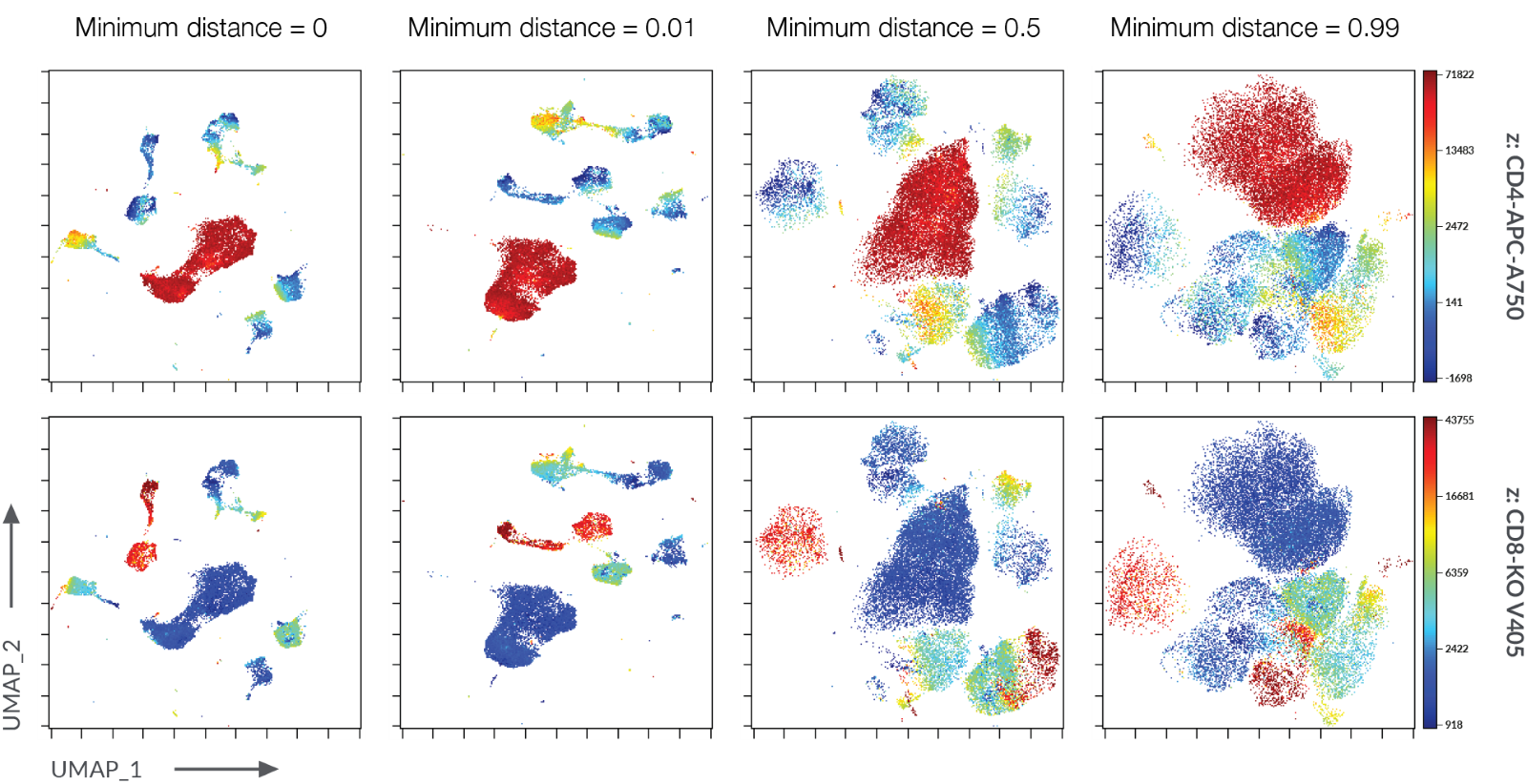
2. Minimum Distance (min_dist): This setting controls the density of points in the low-dimensional representation. A higher value results in a more spread-out embedding, emphasizing separation between clusters. Conversely, a lower value leads to a denser embedding, revealing finer details within clusters.

3. Metric: UMAP offers a wide array of distance metrics to measure the similarity between data points. The choice of metric directly impacts the neighborhood graph construction and, consequently, the embedding. Common metrics include Euclidean distance, Manhattan distance, and cosine similarity.

4. Number of Components (n_components): This setting determines the dimensionality of the output embedding. Choosing an appropriate number of components is crucial for balancing dimensionality reduction with preserving relevant information.

5. Random State: UMAP employs random sampling during the neighborhood graph construction. Specifying a random state ensures reproducibility of the embedding, allowing for consistent results across multiple runs.

Beyond the Basics: Exploring Advanced Settings

UMAP offers a range of advanced settings that provide finer control over the embedding process. These settings cater to specific data characteristics and analysis goals.

1. Metric Keyword Arguments: UMAP allows for customizing the metric used for distance calculation by providing additional keyword arguments. This feature enables tailoring the metric to specific data types or requirements.

2. Transform: UMAP offers different transformations to apply to the data before embedding. These transformations can improve the embedding quality by addressing specific data characteristics, such as scaling or normalization.

3. Init: UMAP provides options for initializing the embedding process. Using a pre-existing embedding as an initial guess can significantly speed up the embedding process, particularly for large datasets.

4. Spread: This setting controls the relative spread of points in the low-dimensional representation. A higher value emphasizes separation between clusters, while a lower value prioritizes preserving local details.

5. Negative Sample Rate: UMAP employs negative sampling to learn the manifold structure. This setting controls the ratio of negative samples to positive samples used during the learning process.

Understanding the Impact of UMAP Settings: A Practical Approach

The choice of UMAP settings depends heavily on the specific dataset and the intended analysis. Experimentation and careful consideration of the data characteristics are crucial for achieving optimal results.

Tips for Effective UMAP Configuration:

• Start with default settings: Begin by exploring the data using UMAP’s default settings to gain an initial understanding of the data structure.
• Adjust n_neighbors and min_dist: Experiment with different values for these parameters to fine-tune the balance between global and local structures.
• Select an appropriate metric: Choose a metric that aligns with the data characteristics and the desired similarity measure.
• Iteratively refine settings: Adjust the settings iteratively based on the resulting embedding and the desired outcome.
• Visualize the embedding: Visualize the embedding to assess the quality of the representation and identify potential issues.

Frequently Asked Questions

Q: How do I choose the optimal number of neighbors for my dataset?

A: The optimal number of neighbors depends on the density of the data and the desired level of detail. Start with a small value (e.g., 5-10) and gradually increase it until the embedding captures the desired structure.

Q: What is the purpose of the min_dist parameter?

A: The min_dist parameter controls the density of points in the embedding. A higher value results in a more spread-out embedding, potentially emphasizing separation between clusters. A lower value leads to a denser embedding, revealing finer details within clusters.

Q: When should I use a different metric than Euclidean distance?

A: Consider using a different metric when Euclidean distance is not suitable for measuring similarity between data points. For example, use cosine similarity for data represented as vectors in a high-dimensional space.

Q: How can I interpret the embedding generated by UMAP?

A: Visualize the embedding using scatter plots or other visualization techniques. Analyze the distribution of points, identify clusters, and interpret the relationships between data points based on their proximity in the embedding.

Conclusion

UMAP, with its flexible settings and powerful capabilities, provides a valuable tool for dimensionality reduction. By carefully selecting and adjusting these settings, researchers and analysts can effectively explore complex datasets, uncover hidden patterns, and extract meaningful insights. Understanding the nuances of UMAP settings empowers users to tailor the embedding process to their specific needs and achieve optimal results in their data analysis endeavors.

Closure

Thus, we hope this article has provided valuable insights into Navigating the Landscape of Dimensionality Reduction: A Comprehensive Guide to UMAP Settings. We hope you find this article informative and beneficial. See you in our next article!